How to Make Models Reason
How to Make Model “Reason” with Group Relative Policy Optimization (GRPO)
You’ll notice that ChatGPT has a small “Reasoning” button under the prompt and see that it suddenvly significantly “evolves” into a more powerful version that can math and coding problem well. Given the recent rise of reasoning powered LLMs, such as OpenAI’s o1 and o3 and DeepSeek’s R1, and some might get curious on how these models are created and trained.
These questions can be:
- What is the methodology to train such reasoning models?
- What difference does it have compared to traditional LLM training process?
In this blog, we will explore the foundational blocks of training/tuning an LLM model to reason and try to answer questions we discussed earlier. The topics would roughly include:
- Introduction to Reinforcement Learning
- Policy in Reinforcement Learning
- PPO (Proximal Policy Optimization)
- GRPO (Group Relative Policy Optimization)
Let us break it down for you.

Post-Training
In the context of training an LLM, we normally think of pretraining -> finetuning -> RLHF (reinforcement learning with human feedback). The latter parts of the LLM training process are called post-training (i.e. the process after pretraining).
A Gentle Introduction to Reinforment Learning
Basically, reinforcement learning is a process of teaching an agent, which can be a language model or any other modality model, on how to behave (take which action) in a given environment setting to maximize certain reward.
Think of how we learn from our past experiences. This can be lessons learned from our mistakes and successes. Through each outcome of our actions, we get certain reward- or punishment (we’ll refer to this as negative or positive feedback). So reinforcement learning is a very natural way of teaching an agent, though the environment is “a bit” more restrained like a sandbox, compared to our real open world.
What’s more interesting about reinceforcement learning, especially when comparing it to machine learning (supervised, using labeled dataset), is that we are not necessarily supervising the model- or an “agent” as we normally refer to in the reinforcement context. We are leaving the agent to learn by itself on how to maximize the reward for every action it takes. The goal is not to micromanage- by telling our baby agent what you did was good or bad- instead, let it observe the outcome itself and learn the best action (let it decide) for each environment state given.
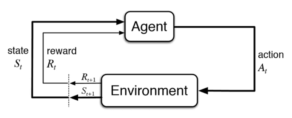
Refer to this flow diagram. The process of reinforcement learning goes like this. Focus!
- Our agent that we want to train receives an environment “state,” denoted as \(S_t\) at time \(t\).
- Based on the state \(S_t\), the agent will take a certain action, denoted as \(A_t\).
- Now, that action will have an impact on the state, which will create a new state of the environment, \(S_{t+1}\).
- Based on the action and the new state, a new reward, \(R_{t+1}\), is calculated- which will influence how the agent will act in subsequent steps.
- Repeat steps 1-4, but for \(t>0\), the agent receives the environment state and reward instead of just the environmnt on \(t=0\).
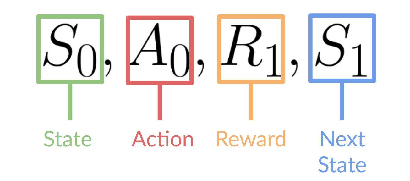
Figure to clarify the notations.
And as described above, the action taken by the agent on time \(t+1\) only depends on the reward and the state of time \(t+1\), which is the new state and reward gained through the action taken right before, i.e. \(A_t\). This is called the Markov Decision Process (MDP), simply put, the agent only needs the current state to decide the best action and neet not the history of all states seen before.
Naturally, the goal of reinforcement learning becomes maximizing the expected cumulative reward.
We can try to assert that the expected cumulative reward can be written as:
\[R(\tau)=\sum^{\infty}_{k=0}r_{t+k+1}\]where \(\tau\) is the trajectory of the state and actions throughtout time like \(\tau=(s_0,a_0,s_1,a_1,...)\).
Keep in mind that since the reward into the future is less likely to occur, we introduce a discount factor to the individual reward, called gamma (\(\gamma\)) that is between \(0\) and \(1\).
So the adjusted expected cumulative rewards becomes:
\[R(\tau)=\sum^{\infty}_{k=0} \gamma^t r_{t+k+1}\]Policy
We noted that the goal of RL is to build an RL agent that can select the actions that maximize its expected cumulative reward.
Then how can a model decide which action to take when given a state? -> policy \(\pi_\theta\).
We can define the “policy” as a parameterized function with respect to \(\theta\) and returns the most optimal action.
\[\text{state}\rightarrow\pi(\text{state})\rightarrow\text{action}\]So naturally our goal becomes to optimizing the policy of the model through training, to get \(\pi^*\), that maximizes the expected reward.
There are mainly two ways to train the RL agent:
- Policy-based optimization: teaching the agent which action to take given the state. It’s direct.
- Value-based optimization: teaching the agent which state is more favorable so the agent takes actions that lead to more favorable states. Indirect.
Since the method that we are curious about today, GRPO, is a policy-based method, let’s talk a bit more about policy-based optimization.
Policy-Based Methods
Simply put, we are optimizing the policy for the agent which can map each environment state to the best corresponding action. This is deterministic, so we can also define a stochastic function that can map each state to a distribution of possible actions.
- Deterministic: \(a=\mu_\theta(s)\). Same state will yield same action.
- Stochastic: \(a\sim\pi_\theta(A\|s)\) is the proabability of taking action \(a\) over probability distribution of the set of possible actions \(A\), given the state.
Now, that we established the policy function, we can write the expected return \(J(\pi)\) as:
\[J(\theta)=E[\sum^T_{t=0}R(s_t,a_t);\pi_\theta]=\sum_\tau P(\tau;\theta)R(\tau)\]where \(P(\tau;\theta)\) is the probability of \(T\)-step trajectory \(\tau\), given \(\theta\).
Since our goal is to maximize \(J(\theta)\), the optimal policy \(\pi^*\) can be expressed as:
\[\pi^*=\argmax_\theta J(\theta)\]Policy Gradient
Great, but how do we actually find this optimal policy \(\pi^*\)?
Assuming that you are familiar with gradient descent, we can apply almost exactly the same method for policy optmization!
We could update our policy by applying gradient to its parameter \(\theta\) as such:
\[\theta_{t+1}=\theta_t+\alpha\nabla_\theta J(\theta)\]The term \(\nabla_\theta J(\theta)\) is the policy gradient.
To make \(J\) differentiable, let’s rewrite our objective function \(J\) as:
\[J(\theta)=E[r(\tau)]=\sum_\tau P(\tau;\theta)R(\tau)=\int\pi_\theta(\tau)r(\tau)d\tau\]over a continuous trajectory \(\tau\).
Now, the policy gradient becoms:
\[\nabla_\theta J(\theta)=\int\nabla_\theta\pi_\theta(\tau)r(\tau)d\tau=\int\pi_\theta(\tau)\nabla_\theta\log\pi_\theta(\tau)r(\tau)d\tau=E[\nabla_\theta\log\pi_\theta(\tau)r(\tau)]\]since \(E[f(x)]=\int p(x)f(x)dx\), refer to the expected value of a continuous random variable with probability density function \(p(x)\).
The idea with Proximal Policy Optimization (PPO) is that we want to improve the training stability of the policy by limiting the change you make to the policy at each training epoch: we want to avoid having too large of a policy update.
For two reasons:
- We know empirically that smaller policy updates during training are more likely to converge to an optimal solution.
- A too-big step in a policy update can result in falling “off the cliff” (getting a bad policy) and taking a long time or even having no possibility to recover.
Mathematical reasoning poses a significant challenge for language models due to its complex and structured nature. In this paper, we introduce DeepSeekMath 7B, which continues pre-training DeepSeek-Coder-Base-v1.5 7B with 120B math-related tokens sourced from Common Crawl, together with natural language and code data. DeepSeekMath 7B has achieved an impressive score of 51.7% on the competition-level MATH benchmark without relying on external toolkits and voting techniques, approaching the performance level of Gemini-Ultra and GPT-4. Self-consistency over 64 samples from DeepSeekMath 7B achieves 60.9% on MATH. The mathematical reasoning capability of DeepSeekMath is attributed to two key factors: First, we harness the significant potential of publicly available web data through a meticulously engineered data selection pipeline. Second, we introduce Group Relative Policy Optimization (GRPO), a variant of Proximal Policy Optimization (PPO), that enhances mathematical reasoning abilities while concurrently optimizing the memory usage of PPO.